Simulation of a Bouncing Ball

bouncing ball simulink example
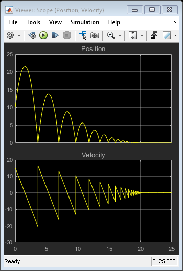
Figure 1: A ball is thrown up with a velocity of 15 m/s from a height of 10 m.
A bouncing ball model is a classic example of a hybrid dynamic system. A hybrid dynamic system is a system that involves both continuous dynamics, as well as, discrete transitions where the system dynamics can change and the state values can jump. The continuous dynamics of a bouncing ball is simply given by:
![]()
![]()
where ![]() is the acceleration due to gravity, x(t) is the position of the ball and v(t) is the velocity. Therefore, the system has two continuous states: position x and velocity v.
is the acceleration due to gravity, x(t) is the position of the ball and v(t) is the velocity. Therefore, the system has two continuous states: position x and velocity v.
The hybrid system aspect of the model originates from the modeling of a collision of the ball with the ground. If one assumes a partially elastic collision with the ground, then the velocity before the collision, v–, and velocity after the collision, v+, can be related by the coefficient of restitution of the ball,  , as follows:
v+=-kv– , x=0
The bouncing ball therefore displays a jump in a continuous state (velocity) at the transition condition, x=0
A bouncing ball is one of the simplest models that shows the Zeno phenomenon. Zeno behavior is informally characterized by an infinite number of events occurring in a finite time interval for certain hybrid systems. As the ball loses energy in the bouncing ball model, a large number of collisions with the ground start occurring in successively smaller intervals of time. Hence the model experiences Zeno behavior. Models with Zeno behavior are inherently difficult to simulate on a computer, but are encountered in many common and important engineering applications.
Using Two Integrator Blocks to Model a Bouncing Ball
MATLAB command:
open_system('sldemo_bounce_two_integrators')Run the command by entering it in the MATLAB Command.
You can use two Integrator blocks to model a bouncing ball. The Integrator on the left is the velocity integrator modeling the first equation and the Integrator on the right is the position integrator. Navigate to the position integrator block dialog and observe that it has a lower limit of zero. This condition represents the constraint that the ball cannot go below the ground.
The state port of the position integrator and the corresponding comparison result is used to detect when the ball hits the ground and to reset both integrators. The state port of the velocity integrator is used for the calculation of v+.

To observe the Zeno behavior of the system, navigate to the Solver pane of the Configuration Parameters dialog box. In the ‘Zero-crossing options’ section, confirm that ‘Algorithm’ is set to ‘Nonadaptive’ and that the simulation ‘Stop time’ is set to 25 seconds. Run the simulation.
Observe that the simulation errors out as the ball hits the ground more and more frequently and loses energy. Consequently, the simulation exceeds the default limit of 1000 for the ‘Number of consecutive zero crossings’ allowed. Now navigate to the Configuration Parameters dialog box. In the ‘Zero-crossing options’ section, set the ‘Algorithm’ to ‘Adaptive’. This algorithm introduces a sophisticated treatment of such chattering behavior. Therefore, you can now simulate the system beyond 20 seconds. Note, however, the chatter of the states between 21 seconds and 25 seconds and warning from Simulink about the strong chattering in the model around 20 seconds.
Using a Second-Order Integrator Block to Model a Bouncing Ball
MATLAB command:
open_system('sldemo_bounce')You can use a single Second-Order Integrator block to model this system. The second equation dx/dt=v is internal to the Second-Order Integrator block in this case. Navigate to the Second-Order Integrator block dialog and notice that, as earlier, x has a lower limit of zero. Navigate to the Attributes tab on the block dialog and note that the option ‘Reinitialize dx/dt when x reaches saturation’ is checked. This parameter allows us to reinitialize dx/dt (v in the bouncing ball model) to a new value at the instant x reaches its saturation limit. For the bouncing ball model, this option therefore implies that when the ball hits the ground, its velocity can be set to a different value, i.e., to the velocity after the impact. Notice the loop for calculating the velocity after a collision with the ground. To capture the velocity v– of the ball just before the collision, the dx/dt output port of the Second-Order Integrator block and a Memory block are used. v– is then used to calculate the rebound velocity v+.


Navigate to the Solver pane of the Configuration Parameters dialog box. Confirm that ‘Algorithm’ is set to ‘Nonadaptive’ in the ‘Zero-crossing options’ section and the simulation ‘Stop Time’ is set to 25 seconds. Simulate the model. Note that the simulation encountered no problems. You were able to simulate the model without experiencing excessive chatter after t = 20 seconds and without setting the ‘Algorithm’ to ‘Adaptive’.
Second-Order Integrator Model Is the Preferable Approach to Modeling Bouncing Ball
One can analytically calculate the exact time  when the ball settles down to the ground with zero velocity by summing the time required for each bounce. This time is the sum of an infinite geometric series given by:
![]()
![]()
Here x0 and v0 are initial conditions for position and velocity respectively. The velocity and the position of the ball must be identically zero for t>t*. In the figure below, results from both simulations are plotted near t*. The vertical red line in the plot is t* for the given model parameters. For t>t* and far away from t*, both models produce accurate and identical results. Hence, only a magenta line from the second model is visible in the plot. However, the simulation results from the first model are inexact after t*; it continues to display excessive chattering behavior for t>t*. In contrast, the second model using the Second-Order Integrator block settles to exactly zero for t>t*.

Figure 2: Comparison of simulation results from the two approaches.
Figure 2 conclusively shows that the second model has superior numerical characteristics as compared to the first model. The reason for the higher accuracy associated with the Second-Order Integrator model is as follows. The second differential equation dx/dt=v is internal to the Second-Order Integrator block. Therefore, the block algorithms can leverage this known relationship between the two states and deploy heuristics to clamp down the undesirable chattering behavior for certain conditions. These heuristics become active when the two states are no longer mutually consistent with each other due to integration errors and chattering behavior. You can thus use physical knowledge of the system to alleviate the problem of simulation getting stuck in a Zeno state for certain classes of Zeno models.